


How to calculate surface magnetism
Magnetic induction intensity, commonly known as surface magnetism, is a key indicator for measuring the performance of magnetic steel. It refers to the magnetic field strength on the surface of the magnetic steel. In many technological fields that require the use of space magnetic fields, the magnetic induction intensity of surface magnetism or specific points is often considered a key technical specification. It should be noted that surface magnetism has directionality, and the numerical value usually refers to the surface magnetism perpendicular to the magnetic pole surface.
So, can the magnetic field be calculated? If possible, what should we do?
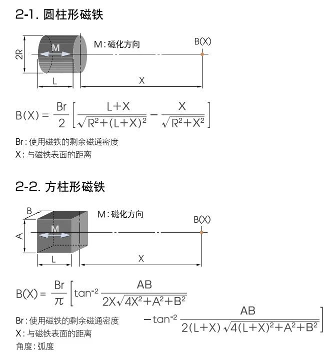
This is a question that many people are interested in. On the internet, we can find some calculation formulas, and many official websites of magnetic material manufacturers also provide calculation tools to facilitate users' calculations. However, those who have used these tools may find that these formulas or tools typically only calculate the surface magnetism of cylindrical and rectangular shaped magnets, and only calculate the surface magnetism at the center position.
Does the calculation become complicated for magnets of other shapes? Has the calculation of the highest magnetic field also become difficult? Indeed, accurately calculating table magnetism is a highly challenging and complex task. For cylindrical and rectangular magnets, we usually assume that the magnetic field distribution is ideal and symmetrical, and the surface magnetic field at the center position is considered to be perpendicular to the magnetic pole surface in an ideal state. The magnetic permeability in the air gap and the magnetic permeability of the magnet are assumed to be equal and have a value of 1.0. Based on these assumptions, we can obtain relatively simple calculation methods. You can refer to the calculation formula provided by TDK for calculation.
As a key indicator for measuring the performance of magnetic steel, the accuracy of its measurement and calculation is crucial for application fields. Although Excel calculators based on theoretical formulas provide convenience for calculations, in practical applications, it is often found that there are significant differences between calculated values and measured values. Taking the N50 D10 * 10mm magnet as an example, even under ideal conditions using a Gaussian meter for measurement, the measured value is difficult to reach the theoretical calculation value. This situation raises questions about the accuracy of the calculation formula.
To gain a deeper understanding of this issue, we need to review the applicable conditions and assumptions of the formula. Firstly, the value of X in the formula represents the distance from the calculation point to the surface of the magnet. Although in practical operation, we try to make the measuring probe closely adhere to the surface of the magnet as much as possible, the protective shell of the probe will introduce some errors. For example, the Hall chip of the commonly used Japanese KANETEC Gaussian meter probe is covered with a transparent protective shell about 0.2mm thick. In addition, the coating on the surface of the finished magnet will also have a shielding effect on the magnetic field, resulting in a decrease in the measured value. For example, the thickness of nickel copper nickel coating is generally 0.02mm, which can affect the magnetic field. Therefore, in actual measurements, the X value needs to be additionally compensated by 0.4-0.5mm to more accurately reflect the actual situation.
However, another important factor that affects the measurement results is the magnetic permeability of the magnet and the air gap. In theory, the formula assumes that the magnetic permeability of both the magnet and the air gap is equal to 1.0. Although the permeability of air is very close to 1.0, the permeability of magnets is often higher, especially N series and M series neodymium iron boron magnets, whose permeability often exceeds 1.05, and some even reach 1.1. The difference in magnetic permeability can affect the distribution and intensity of the magnetic field, thereby affecting the measurement data.
To fully understand the impact of magnetic permeability on test data, we need to return to the concept of demagnetization curve:
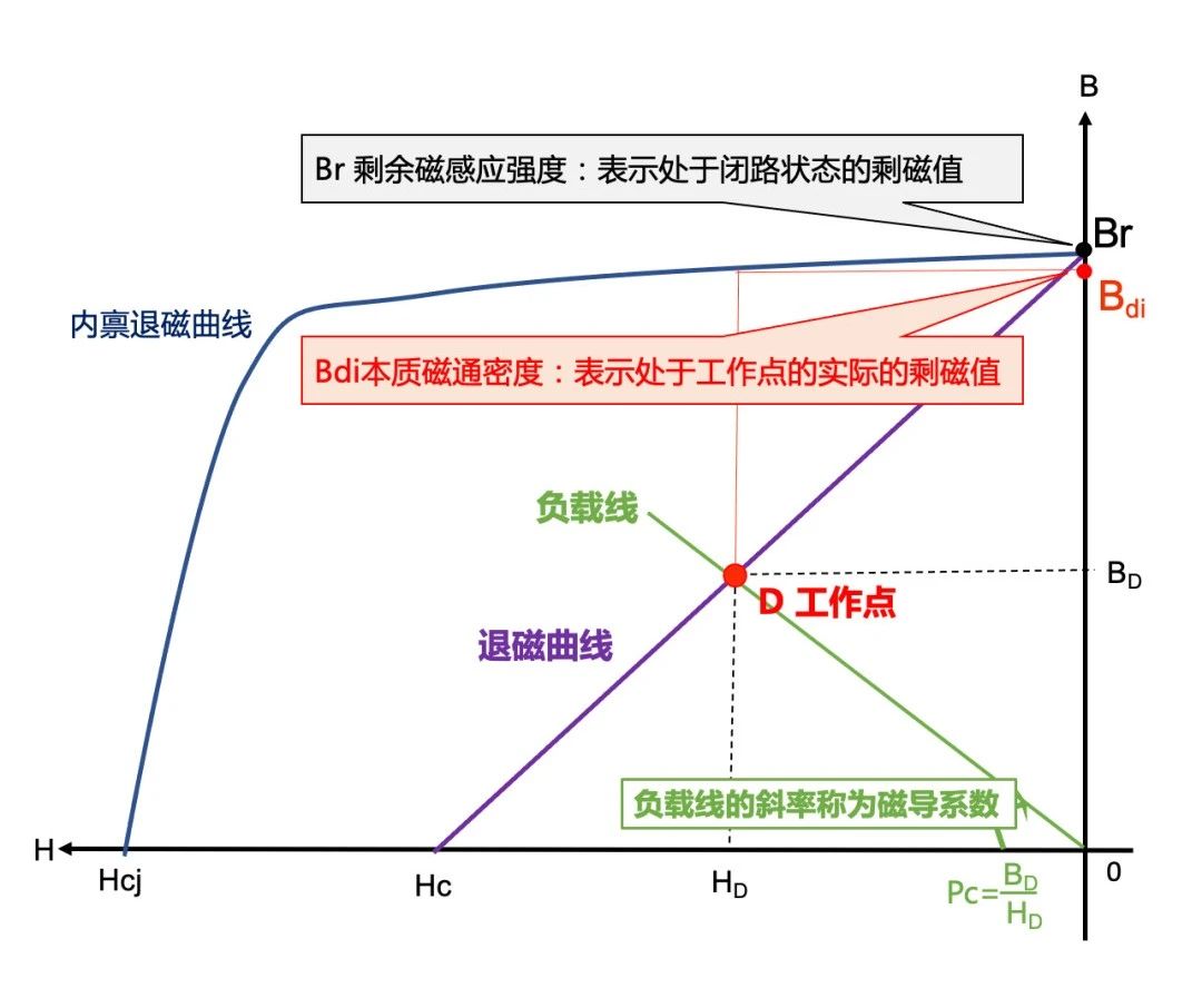
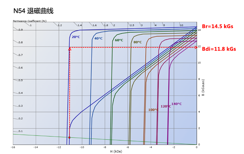
From the demagnetization curve, it can be seen that the actual remanence value of a magnet in an open circuit state is not the ideal Br value, but lower than Br, which we call the intrinsic magnetic flux density Bdi. The reason for this is that the initial state of the blue J-H demagnetization curve is not ideally parallel to the X-axis, but inclined. Therefore, the Br value will definitely be greater than Hcb, and the recovery magnetic permeability μ rec=Br/Hcb cannot be 1.0. There is also a situation where the B-H line has a turning point, and the working point of the magnet is below the turning point, so the actual Bdi will be much lower than Br, and the calculated result will deviate more from the actual value, as shown in the figure below. This also explains why the actual center surface magnetic field of the N54 20 * 10 * 1mm magnet is not only much lower than the theoretical calculation value, but also very unstable
Please note that the formula mainly applies to permanent magnet materials with linear demagnetization characteristics, such as neodymium iron boron, samarium cobalt, and ferrite. For permanent magnetic materials with nonlinear demagnetization curves, such as aluminum nickel cobalt, iron chromium cobalt, and various soft magnetic materials, these formulas are not applicable. In addition, these calculation methods are also not applicable to oblique magnets whose magnetization direction is not perpendicular to the magnetic pole surface.